How To Trade Cross-Market Statistical Arbitrage On Prediction Markets (Complete Quant Roadmap)

I'm going to break down exactly how quantitative hedge funds exploit structural price discrepancies between competing prediction platforms (like Polymarket and Kalshi) to lock in riskless alpha 👇

I'm also releasing a public repository and a 55GB dataset containing tick-by-tick order book L2 snapshots going back to late 2024.

---

The L2 Order Book Dataset Is Now Public

Most retail traders look at historical transaction prices (Charts). Quant funds look at the limit order book (L2).

When an event is traded simultaneously across platforms, temporary liquidity imbalances create deterministic price gaps. To backtest these inefficiencies, you need the depths of the bid-ask queues, not just the execution prints.

This dataset includes:

• Full L2 order book snapshots (up to 20 levels deep) sampled at 100ms intervals.
• Cross-platform synced timestamps.
• Over 850 million state updates stored in highly optimized Apache Parquet format.

Before we dive into the predictive mathematics, let's get your local environment configured to handle institutional-grade order book analytics.

---

How to Set Up the Dataset (Step by Step)

Prerequisites:

• Python 3.10 or higher
• 60GB of unallocated SSD disk space
• Terminal (Mac/Linux) or PowerShell (Windows)

Step 1: Install uv (Blazing Fast Dependency Manager)

# On Mac/Linux
curl -LsSf https://astral.sh/uv/install.sh | sh

# On Windows (PowerShell)
irm https://astral.sh/uv/install.ps1 | iex

Step 2: Clone the Quantitative Arbitrage Repository

git clone https://github.com/Jon-Becker/prediction-market-analysis
cd prediction-market-arbitrage

Step 3: Synchronize Virtual Environment and Dependencies

uv sync

This deterministically provisions an isolated environment with polars, scikit-learn, statsmodels, and high-performance analytical extensions.

Step 4: Stream and Extract the Compressed L2 Order Book Data

make download-ob

This pulls orderbooks_l2.tar.zst (39GB compressed) from a high-throughput Cloudflare R2 bucket and decompresses it natively into your local directory.

Step 5: Verify Dataset Integrity

ls data/snapshots/polymarket/
ls data/snapshots/kalshi/

If configured correctly, you will see daily Parquet files split by market category. You are now sitting on the exact data infrastructure used by systematic trading desks.

---

How Hedge Funds Capitalize on This Data

Retail traders wait for news to break, buy a contract, and pray they guessed right.

Hedge funds don't care who wins an election, an award, or an economic release. They treat prediction markets as a network of fragmented order books. They exploit mathematical cointegration and order flow imbalances to trade the spread between platforms, delta-hedging their inventory to zero.

Here are the two primary algorithmic methodologies deployed on this data.

---

Method 1: Cointegration and the Ornstein-Uhlenbeck Mean-Reversion Framework

When two distinct platforms host markets on the exact same real-world outcome, their long-term prices must converge to identical terminal values ($1.00 or $0.00).

However, local liquidity shocks (e.g., a whale dumping $500k of contracts on one platform) cause temporary divergence. We model this relationship using statistical cointegration.

Phase 1: Testing for Cointegration

Let P_{P,t} be the mid-price of the contract on Polymarket at time t, and P_{K,t} be the mid-price on Kalshi. We construct a linear combination representing the spread S_t:

> S_t = P_{P,t} - β * P_{K,t} - μ

Where β is the cointegration coefficient and μ is the constant intercept. Quant funds run the Augmented Dickey-Fuller (ADF) test or the Johansen test on the historical Parquet files to confirm that Sₜ is a stationary time series (I(0)), meaning it consistently reverts back to its mean.

---

Phase 2: Modeling the Continuous Spread Dynamics

Once cointegration is statistically validated, we model the continuous-time evolution of the spread using an Ornstein-Uhlenbeck (OU) stochastic process:

> dSₜ = θ(μ − Sₜ)dt + σ dWₜ

Where:

• θ represents the rate of mean reversion (how fast the price gap closes).

• μ is the long-term mean of the spread.

• σ is the historical volatility of the spread.

• dWₜ is a standard Brownian motion increment representing random market noise.

---

Phase 3: Analytical Calibration via Maximum Likelihood Estimation (MLE)

By applying the Euler–Maruyama discretization to our historical data over a sampling interval Δt\Delta tΔt, we transform the continuous equation into a trackable regression model:

> S_ti​​=S_ti−1​​e−θΔt+μ(1−e−θΔt)+εt​

Using Maximum Likelihood Estimation on the 850-million-row dataset, funds extract the exact numerical value of θ. If θ implies a mean-reversion time

> τ=1\θ

faster than the platform’s execution latency, the asset is deemed highly tradeable.

---

Phase 4: Constructing Optimal Entry and Exit Thresholds

An amateur trader enters an arbitrage as soon as a gap appears. A quant desk solves an optimal stopping problem. Using the calibrated OU parameters, the optimal entry thresholds x_open and exit thresholds x_close are derived to maximize the expected return per unit of time:

> Maximize E [ e^{-τ τtrade(S_t_close - S_t_open - c)} / τ_trade

Where c represents the linear transaction fees plus slippage incurred across both venues, and r is the continuous risk-free rate.

Spread (S_t)
        ^
        |       ============== Optimal Short Entry (+x_open)
        |     / \
  ------|----/---\-------/---------------- Long-Term Mean (μ)
        |   /     \     /
        |  /       \___/  ==== Optimal Long Entry (-x_open)
        +-----------------------------------> Time (t)

---

Method 2: Order Book Imbalance (OBI) and High-Frequency Micro-Price Prediction

At millisecond horizons, macro cointegration models are too slow. To front-run short-term price movements across venues, funds look directly at the liquidity distribution via Order Book Imbalance (OBI).

Phase 1: Mathematical Definition of Imbalance

The standard mid-price ignores the volume available at the inside market. If the best bid has 100,000 contracts and the best ask has only 1,000 contracts, the price is mathematically heavily pressured to move upward.

We quantify this utilizing the Level 1 OBI metric:

> I_t​=(V_b​(t)−V_a​(t)) / (V_b​(t)+V_a​(t))​, I_t​∈[−1,1]

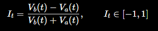
Where V_b(t)is the volume available at the best bid price (P_b), and V_a(t) is the volume available at the best ask price (P_a).

Phase 2: Micro-Price Formulation

To calculate the "true" instantaneous value of a contract before a transaction prints, funds compute the Micro-Price (P_micro), weighting the bid and ask prices inversely by their structural volume:

> P_micro​(t)=V_b​(t)P_a​(t)+V_a​(t)P_b​(t)​ / V_b​(t) + V_a​(t)

By substituting the imbalance definition into the micro-price equation, we reveal its linear dependency on order book structure:

> P_micro​(t)=P_mid​(t)+I_t​(Δspread / 2​​)

Where

> P_mid​(t)=P_a​(t)+P_b​(t)​ / 2

and

> Δspread​=P_a​(t)−Pb_​(t)

Phase 3: Cross-Venue Predictive Signaling

The real alpha emerges when you map P_micro cross-platform.

Because Polymarket is fully on-chain/hybrid and Kalshi is a centralized regulatory clearinghouse, their API architectures process order flow at inherently different velocities.

> ΔP_Kalshi​(t+δ)=f(I_Polymarket​(t),P_micro, Polymarket​(t)−P_micro, Kalshi​(t))

Quant desks compute a rolling Markov chain transition matrix over the historical Parquet data. They measure the probability that a significant imbalance shift (I > 0.8) on Platform A predicts a clearing of the ask book on Platform B within a δ = 200ms window.

If the predictive probability exceeds a structural threshold, automated execution systems immediately cross the spread on the lagging exchange, capturing the price adjustment before retail order routers even register the shift.

---

Process Over Prediction

The core takeaway is simple: institutional trading desks are completely agnostic to the actual underlying events. They do not read political polling data, they do not analyze macroeconomic reports, and they do not have a specialized opinion on the future.

Their unfair advantage resides entirely within operational process and structural math:

• Continuous Risk Harmonization: Calibrating positions through empirical Ornstein-Uhlenbeck parameters rather than nominal price spreads.
• Microstructure Dominance: Exploiting the mathematical relationship between multi-venue order book imbalances and micro-price variations.
• Latency Capitalization: Running execution engines optimized to act on cross-platform predictive signals before the retail UI can refresh.

The open-source repository and the 55GB Parquet dataset provide the exact testing sandbox required to build, test, and execute these frameworks natively.

---

> Save it to your bookmarks so you don't lose it 📝