QUANT PHYSICS: How Hedge Funds Actually Turn Chaos Into Probability

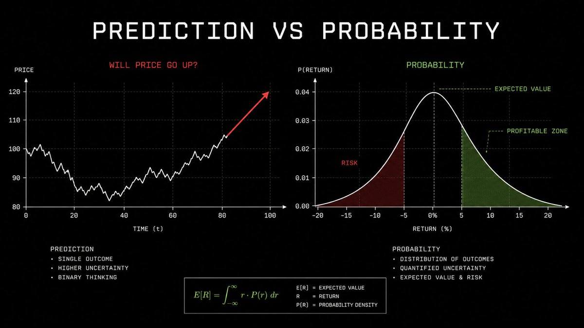
Most people look at a chart and ask one question:

> Will it go up or down?

Quant funds ask a different one:

> What is the probability distribution of outcomes, how much can we lose if we are wrong, and is the expected return worth taking the trade?

That difference sounds small.

It is not.

One approach needs a prediction.

The other needs a system that survives being wrong many times.

Markets are chaotic because millions of people, funds, bots, options desks, liquidations, earnings reports, interest-rate decisions, and random headlines all hit the same order book at once.

But chaotic does not mean completely random.

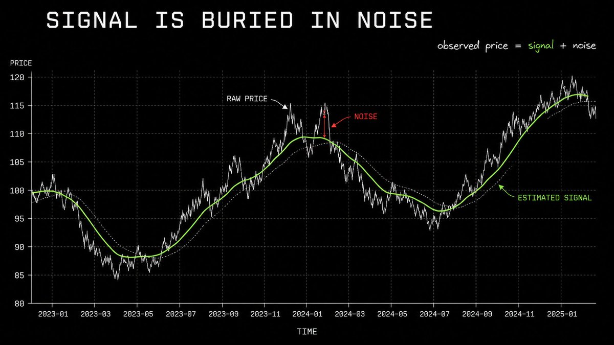
It means the signal is buried under noise.

Quant research is the attempt to find those small, repeatable patterns without lying to yourself about how fragile they are.

The First Rule: Hedge Funds Do Not Need To Predict The Next Candle

A quant strategy can be profitable while being wrong on most individual trades.

That sounds impossible until you stop thinking in predictions and start thinking in expected value.

Expected Value =
(probability of winning × average win)
−
(probability of losing × average loss)

Imagine a strategy that wins only 45% of the time.

Sounds bad.

But if its average winning trade is +3% and its average losing trade is -1%, the system can still make money over a large enough sample.

That is the core idea.

The fund is not asking:

> “Am I certain Bitcoin goes up this week?”

It is asking:

> “Given volatility, funding, liquidity, options positioning, historical behaviour, and current market regime, is this trade priced incorrectly enough to justify the risk?”

A quant does not need omniscience.

It needs a small edge that remains after fees, slippage, bad fills, and the inevitable trades that go wrong.

This is why serious funds care so much about risk models.

A strategy that looks brilliant in a calm market can become dangerous the moment volatility changes, liquidity disappears, or many supposedly independent trades suddenly become correlated.

Research on hedge-fund tail risk has found that strategy sensitivities can rise sharply during periods of market distress. In plain English: assets and strategies that looked uncorrelated in normal conditions can start losing together when it matters most.

A Strategy Can Be Wrong More Often Than It Is Right

A quant strategy does not need a 90% win rate.

It needs a positive expected value after losses, fees, and bad execution.

Here is a simplified example.

WIN RATE: 46%

AVERAGE WIN: +1.6R
AVERAGE LOSS: -1.0R

EXPECTANCY PER TRADE:

(0.46 × 1.6R) − (0.54 × 1.0R)
= 0.736R − 0.540R
= +0.196R

If 1R is the amount you are willing to lose on one trade, the strategy earns an expected +0.196R per trade.

Over 100 trades:

100 × 0.196R = +19.6R expected value

That does not mean the strategy makes money every week.

It means the process has an edge only if the sample is large enough and the execution is real.

A system with a lower win rate can outperform a system that “wins all the time” but occasionally loses ten times more than it makes.

Markets Behave More Like Weather Than Like A Slot Machine

The easiest wrong analogy is a slot machine.

A slot machine has fixed rules. Every pull is almost independent from the last.

Markets are different.

They have memory.

Not necessarily in the simple form of “price went up yesterday, so it goes up today.”

But in the form of volatility, liquidity, positioning, attention, and stress.

A quiet market tends to remain relatively quiet for a while.

A violent market tends to remain violent for a while.

That phenomenon is called volatility clustering.

Large price moves tend to arrive near other large price moves. Calm periods cluster too.

This is one of the most established “stylized facts” of financial markets. Studies of equity markets and high-frequency data repeatedly document volatility clustering, heavy tails, and non-linear dynamics.

Think about it like weather.

A single hot day does not guarantee the next day will be hot.

But a heatwave changes the probability distribution of tomorrow.

Quant funds try to identify these shifts early.

They do not just ask whether price is moving.

They ask what kind of market they are currently in.

Low-volatility regime:
smaller moves
tighter spreads
mean reversion may work better

High-volatility regime:
larger moves
wider spreads
trend-following or defensive positioning may matter more

Stress regime:
liquidity disappears
correlations jump
normal models become unreliable
survival becomes the trade

Volatility Is A Regime, Not A Number

A common mistake is treating volatility as one fixed property of an asset.

It is not.

A 2% daily move means very different things depending on whether the market has recently been moving 0.5% per day or 5% per day.

A rough annualized-volatility calculation is:

ANNUALIZED VOLATILITY
=
DAILY VOLATILITY × √365

For a crypto asset moving roughly 2% per day:

0.02 × √365
= 0.02 × 19.1
= 38.2% annualized volatility

If daily volatility jumps from 2% to 5%:

0.05 × √365
= 95.5% annualized volatility

The price did not merely become “more volatile.”

The entire risk profile of every position changed.

That is why a strategy that used safe leverage in a calm regime can become reckless during a stress regime.

Model 1: Brownian Motion Is The Starting Point, Not The Answer

In physics, Brownian motion describes the unpredictable movement of particles suspended in a fluid.

In finance, it became a useful way to describe a price that receives countless small shocks.

That gave us foundational models such as geometric Brownian motion and, later, the Black-Scholes options framework.

The idea is elegant:

Price tomorrow =
price today
+
random movement
+
a small directional drift

The problem is that real markets are messier than the textbook version.

Real returns do not follow a neat bell curve.

Crashes happen more often than a simple Gaussian model would predict.

Volatility changes over time.

Prices can jump.

Liquidity can vanish in seconds.

A normal distribution tells you that extreme events should be extremely rare.

Markets regularly remind people that “extremely rare” is not the same as impossible.

That is why quant researchers do not stop at Brownian motion.

They add stochastic volatility, jump processes, regime switching, fat tails, and stress testing.

The purpose is not to find a perfect model.

There is no perfect model.

The purpose is to build a model that fails less catastrophically when reality refuses to behave.

The Textbook Model And The Real Market

The textbook version of price movement is often written as:

$$dS = μSdt + σSdW$$

You do not need to memorize it.

The useful translation is:

PRICE CHANGE
=
EXPECTED DRIFT
+
RANDOM SHOCK

• μ is the expected drift.
• σ is volatility.
• dW is the random shock.

The problem is that the random shock is not always small.

A simple model assumes extreme moves are very rare.

Real markets have jumps, liquidations, forced selling, thin order books, and panic.

That creates fat tails.

NORMAL MODEL:
a 5σ event should be almost impossible

REAL MARKET:
extreme moves occur far more often than
a clean bell curve would suggest

This is why risk teams test portfolios against jumps and regime changes, instead of trusting a smooth distribution alone.

Model 2: Signal Vs Noise

A chart contains information.

It also contains an absurd amount of garbage.

A one-minute candle can move because of:

• one large market order;
• an options hedge;
• a liquidation;
• a market maker rebalancing inventory;
• an ETF flow;
• a rumor;
• an automated arbitrage trade;
• a real change in fundamentals;
• or nothing important at all.

The hard part is that these look similar when you only stare at candles.

This is where quant research starts becoming useful.

A fund collects data and asks whether a feature has predictive value across many observations.

Not one beautiful example.

Not one backtest screenshot.

Not one week where the strategy printed.

Thousands of observations across different market conditions.

For example:

Hypothesis:
Extreme funding rates tend to precede a reversal.

Test:
Collect funding, open interest, price, liquidations,
and volatility across multiple market cycles.

Question:
Does the effect survive fees, slippage,
different exchanges, and out-of-sample testing?

Most hypotheses die here.

That is not failure.

That is the research process working.

The dangerous trader sees a pattern three times and calls it an edge.

The quant sees the same pattern and asks whether it survives 10,000 attempts to prove it wrong.

Model 3: Entropy And The Cost Of Overtrading

Entropy is often simplified as disorder.

That is close enough for markets.

The more participants react to the same information, copy the same trade, use the same indicators, and chase the same narrative, the more difficult it becomes to extract clean signal from price.

A quant fund is not just trying to find information.

It is trying to find information that is:

• not already fully priced in;
• not too expensive to trade;
• not too crowded;
• not based on data leakage;
• not destroyed by fees;
• not likely to vanish after publication.

This is why many retail strategies look good until they are traded.

A strategy can have a genuine pattern and still be useless.

Maybe the signal appears only once per month.

Maybe entering the trade moves the market against you.

Maybe the exchange fee eats the edge.

Maybe everyone discovered it on the same Twitter thread.

Maybe it worked only because the dataset accidentally included future information.

The model is not the business.

The full execution loop is the business.

Raw idea
→ data
→ clean data
→ hypothesis
→ backtest
→ out-of-sample test
→ execution model
→ risk limits
→ live monitoring
→ post-trade review

Every step removes some of the fantasy.

That is exactly the point.

Model 4: Phase Transitions And Market Crashes

Water does not gradually become ice forever.

At a certain point, the state changes.

Markets can do something similar.

For weeks, everything looks normal:

• volatility is low;
• leverage increases;
• spreads are tight;
• people feel safe;
• correlations look manageable.

Then a trigger arrives.

A surprise macro number.

A depeg.

A forced unwind.

A major liquidation.

A geopolitical headline.

The trigger is not always the real cause.

Sometimes the system was already fragile.

The event simply reveals it.

This is why crashes feel sudden even when the conditions behind them took months to build.

In crypto, this is especially visible because leverage, liquidations, perpetual futures, and public positioning data make the feedback loop easier to observe.

A price drop liquidates long positions.

Those liquidations become forced market sells.

Forced sells push price down further.

That triggers more liquidations.

The market becomes a self-reinforcing system.

This is not magic.

It is market structure.

Recent research on order flow and volatility explicitly models the connection between persistent order flow, market impact, volume, and volatility.

A Simplified Liquidation Cascade

This is not an exchange model.

It is a simplified example of why liquidations can accelerate a move.

Imagine a thin order book.

BID DEPTH:

$100k of buy orders every 0.5% lower

0.0%   → $100k
-0.5%  → $100k
-1.0%  → $100k
-1.5%  → $100k
-2.0%  → $100k

Now imagine a $500k forced market sell.

It consumes five levels of bids.

$500k forced sell
÷
$100k bid depth per level
=
5 order-book levels consumed

If each level is spaced 0.5% apart:

5 levels × 0.5%
=
approximately 2.5% immediate price impact

Now assume that 2.5% move triggers another $1M in leveraged long liquidations.

The original sell did not just move price.

It created more forced sellers.

INITIAL SELL
→ PRICE IMPACT
→ LIQUIDATIONS
→ FORCED SELLS
→ THINNER LIQUIDITY
→ LARGER PRICE IMPACT

That is the feedback loop.

The real numbers differ by asset, exchange, and time of day.

The mechanism does not.

Model 5: Correlation Is Not Constant

One of the biggest traps in finance is assuming diversification works forever.

A portfolio can look diversified when markets are calm.

Then a crisis arrives and everything becomes one trade.

Growth stocks, crypto, venture exposure, leveraged tech, small caps, and “alternative” strategies can all suddenly react to the same underlying force: liquidity leaving the system.

Correlation is not a permanent number.

It changes with regime.

That is why a strategy should not be judged only by its average return.

It should be judged by how it behaves when the environment changes.

A serious risk system asks:

What happens if volatility doubles?

What happens if spreads widen 5x?

What happens if we cannot exit at the backtest price?

What happens if our “independent” positions all fall together?

What happens if the model was trained only on a bull market?

The job is not to eliminate risk.

That is impossible.

The job is to understand which risks you own before the market forces you to discover them.

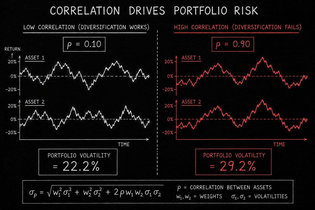
Diversification Can Disappear Exactly When You Need It

Two assets can appear diversified in normal markets.

Then stress arrives and they start moving together.

For an equal-weight portfolio of two assets with the same volatility, portfolio risk is approximately:

$$σp = σ × √(0.5 + 0.5ρ)$$

Assume both assets have 30% annual volatility.

In a calm market, correlation is 0.10

σp = 30% × √(0.5 + 0.5 × 0.10)
σp = 30% × √0.55
σp ≈ 22.2%

In a stressed market, correlation jumps to 0.90

σp = 30% × √(0.5 + 0.5 × 0.90)
σp = 30% × √0.95
σp ≈ 29.2%

Nothing about the two individual assets changed.

But the diversification benefit almost disappeared.

That is why “I own several different coins/stocks” is not necessarily a risk strategy.

The question is whether they remain different when liquidity leaves the market.

What Quant Funds Actually Build

The public imagines a quant fund as one genius, one equation, and one secret model.

The reality is much less cinematic.

A serious quant operation is a stack of systems:

• data ingestion;
• data cleaning;
• research infrastructure;
• portfolio construction;
• execution logic;
• transaction-cost modelling;
• risk controls;
• monitoring;
• human review.

The “signal” might be a small part of the total machine.

In some strategies, execution quality matters more than prediction.

If your expected edge is 10 basis points but poor fills cost 15 basis points, you do not have an edge.

You have an expensive hobby.

This is why quant firms hire across mathematics, physics, statistics, engineering, data infrastructure, and market microstructure.

The model may identify an opportunity.

The system has to capture it before it disappears.

Three Real Quant Mindsets You Can Use Without A Hedge Fund

You do not need a PhD, a colocation server, or a billion-dollar fund to use the useful part of this thinking.

1. Stop Asking For Certainty

Replace:

> “Will this asset go up?”

With:

> “What would have to be true for this setup to work, what would invalidate it, and what is my expected downside if I am wrong?”

That single shift removes a lot of emotional trading.

2. Track The Regime Before The Setup

The same strategy can behave differently in different environments.

A breakout system might work during expansion and fail in a low-volatility chop.

A mean-reversion trade might work in a stable range and get destroyed during a real trend.

Before entering a trade, define the regime:

3. Treat Risk As A Position, Not A Disclaimer

Most people decide position size last.

Quants decide it first.

You can have a good thesis and still lose badly because your sizing was irrational.

A small position in a high-quality trade may be more useful than a huge position in a trade you “feel certain” about.

The market does not care how convinced you were.

Position Sizing Is Where A Thesis Becomes A Risk Decision

Position Sizing Is Where A Thesis Becomes A Risk Decision

Suppose you have a $20,000 portfolio.

You decide the maximum loss on one trade is 1% of capital.

$20,000 × 1%
=
$200 maximum loss

Your trade idea is invalidated if price moves 4% against your entry.

The maximum position size is:

POSITION SIZE
=
MAXIMUM LOSS
÷
STOP DISTANCE

$200 ÷ 4%
=
$5,000 position

Not $20,000.

Not “all-in because the setup looks perfect.”

$5,000.

If the stop is hit, the loss is approximately $200 before fees and slippage.

This is not glamorous.

It is how a bad trade stays a bad trade instead of becoming a portfolio event.

The Part Nobody Wants To Hear

Quant models fail.

They fail because:

• markets evolve;
• participants adapt;
• data is incomplete;
• backtests overfit;
• correlations change;
• liquidity assumptions break;
• a model learns the past too well;
• the future arrives in a different shape.

Even the best framework cannot remove uncertainty.

That is why the useful lesson from quant physics is not:

> “Find the formula that predicts markets.”

It is:

> “Build a process that respects uncertainty better than the average participant.”

The edge is rarely one magic indicator.

It is the discipline of testing ideas, sizing risk, tracking regimes, and accepting that a model can be useful without being permanently true.

VaR Is Useful Until The Market Stops Being Normal

Value at Risk estimates a loss threshold over a chosen time horizon.

A simple one-day 95% VaR approximation:

VaR(95%)
≈
1.65 × portfolio value × daily volatility

For a $50,000 portfolio with 2% daily volatility:

1.65 × $50,000 × 0.02
=
$1,650

Under the model assumptions, there is a 5% chance of losing more than roughly $1,650 in a day.

But that final sentence matters:

> Under the model assumptions.

If volatility spikes, correlations converge, or price gaps through liquidity, the real loss can be far larger.

That is why VaR is a dashboard instrument, not a guarantee.

A risk model is useful when it tells you what it cannot see.

The Quant Physics Playbook

1. Think in distributions, not predictions.

2. Separate signal from noise before risking money.

3. Assume volatility changes in regimes.

4. Treat liquidity as a variable, not a guarantee.

5. Expect correlations to rise when markets panic.

6. Test for fees, slippage, and data leakage.

7. Size trades so that being wrong does not remove you from the game.

8. Review every strategy after market conditions change.

A hedge fund does not turn chaos into certainty.

It turns chaos into a set of measurable probabilities, then decides whether those probabilities are worth owning.

That is a much less exciting promise than “this indicator predicts the next 100x.”

It is also much closer to how real risk is managed.